Varying goals for solar

Cool - I hadn’t looked at rastervis yet, though I have been using his xyplot() package occasionally when I first try to plot an object out of his code. But I’m doing most of my plotting in ggplot2() since it is very predictable and fast.

And the radiation plots are truly cool, though I’m trying to wrap my mind around how you would use these month to month comparisons.

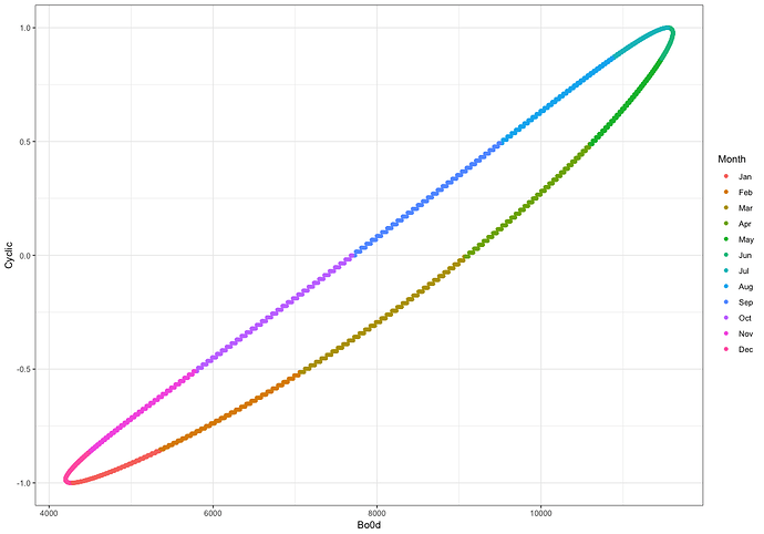
Couldn’t hold myself back… Had to double check my 2 old equations of daily irradiance against the solaR package’s much more sophisticated calculation. Good news, everything seems kosher. My older analysis holds, and Bo0d looks like it takes into account some very small additional tertiary effects beyond H0h. BoD is almost exactly 10000x H0h (just different units).

But the best part is that I now trust my intraday results as well.

solaR Bo0d vs. Cyclic (a simple cosine equation with a period of 365.25 days)

lm(formula = Cyclic ~ Bo0d, data = SolarMix)

Residuals:
     Min       1Q   Median       3Q      Max 
-0.25787 -0.14119  0.05914  0.12754  0.16210 

Coefficients:
              Estimate Std. Error t value Pr(>|t|)    
(Intercept) -2.159e+00  1.009e-02  -214.0   <2e-16 ***
Bo0d         2.637e-04  1.166e-06   226.1   <2e-16 ***
---
Signif. codes:  0 ‘***’ 0.001 ‘**’ 0.01 ‘*’ 0.05 ‘.’ 0.1 ‘ ’ 1

Residual standard error: 0.1455 on 2302 degrees of freedom
Multiple R-squared:  0.9569,	Adjusted R-squared:  0.9569 
F-statistic: 5.113e+04 on 1 and 2302 DF,  p-value: < 2.2e-16

solaR Bo0d vs. my more sophisticated H0d formula

Call:
lm(formula = H0h ~ Bo0d, data = SolarMix)

Residuals:
       Min         1Q     Median         3Q        Max 
-0.0223529 -0.0081799  0.0009893  0.0102988  0.0163886 

Coefficients:
              Estimate Std. Error t value Pr(>|t|)    
(Intercept) -5.767e-02  7.701e-04  -74.89   <2e-16 ***
Bo0d         1.027e-04  8.904e-08 1153.38   <2e-16 ***
---
Signif. codes:  0 ‘***’ 0.001 ‘**’ 0.01 ‘*’ 0.05 ‘.’ 0.1 ‘ ’ 1

Residual standard error: 0.01111 on 2302 degrees of freedom
Multiple R-squared:  0.9983,	Adjusted R-squared:  0.9983 
F-statistic: 1.33e+06 on 1 and 2302 DF,  p-value: < 2.2e-16

And for those of you who know what a Residual is, you can see the extra effects and associated magnitude calculated in Bo0d vs. H0h in this plot…

Time to solve my “wing” problem !

Still sorting out ways to linearize my “wing” more using the SolaR package. I’m now trying to convert from radiation striking the top of the atmosphere to radiation hitting the earth’s surface, then hitting my angled solar panels with about a 20 degree angle west of south orientation. Those factors might just be the reason for the loop pattern.

I have seen a similar kind of loop before when comparing my Sense solar generation vs. my SolarCity generation, where Sense was showing more power being produced in the morning hours vs. Solar city, and the opposite in the afternoon. I eventually tracked down to interval accounting counting being off between the two of them. But the “wings” aren’t as symmetrical around the unity line, so there’s more at play here…

I did do a quick shot at automatically locating the bad points using a simple linear model. First, I removed the 605 missing points (that number dropped from over 1100, because I’m now only looking at daytime data) that were manufactured by me to fill in the gaps. Those were simple because they had their other entries marked as NA. Then I used linear modeling to identify the 400 points with the largest positive residuals. That did a good job finding most of the “shadow wing”. I’m guessing I could now cut the power production for those points in half and stuff that data into the nearest NA or smallest neighbor. All this is under the assumption that SolarCity and the inverter are set up to work around data transmission failures.

I also decided to remove those 400 + 600 points and remodel using a new linear equation. Then I picked off the next 400 points with the highest absolute residual (plus or minus). The next bunch would come from the the bottom.

I also tried one more interesting R package called “robustbase” which offers more robust fitting algorithms that are supposed to deal with bad date. In the case of a linear model, lmrob() iteratively assigns weights to points during regression, giving smaller weights to points with the highest residuals. After a number of remodeling interactions with the weights used in regression, the weights stabilize, and you have your result. I have rounded and multiplied the weights by 10 (usually 0.0-1.0) for annotating the “wing” below. As you can see, this also helps pick off the shadow wing above the wing, as well as low lying power production during high B0 periods (everything 7 and below). But I’m sure that some of the “shadow wing” is still obscured by the good data. Plus weight 7 and 6 data below the wing is probably legit.

OK, time to make some more progress on connecting ground-based measurements with simulated analytic results from solaR. I’ve been stymied a bit by the last stages of solaR that translate top of atmosphere equations/readings for Bo0 to best case and realistic solar production. There are really 3 steps in between:

  • Bo0, geometric, temperature and calibration measurements to earth surface measurements of G0 (GHI - global horizontal irradiance), D0 (DHI - direct horizontal irradiance)
  • From those to Geffective and Deffective, based on the tilt and orientation of my fixed solar install
  • And from those irradiances to actual solar production.
    I really just want to get to Geffective and chart against my solar production. But right now, it’s not clear those steps are working the way I’m trying to use the package.

In the meantime, I dug up some local half-hourly solar measurements for my area courtesy of the NREL NSRDB resource. It’s a 2013 through 2015 record that I can use to compare my data against as well as use to calibrate and even feed solaR, if I can get it working. But for now I’m going to use to make sense of my solar data.

The first thing I attempted to do is chart measured GHI (G0) for this time period against my kWh production during the same period.

Wow ! That looks familiar. Another “wing” pattern. Looks very close to my Bo0 (calculated using solar geometry) vs. kWh, though a little more diffuse since it only contains 50K points instead of the 225K points in the original (the measured data is only half the data period and half the sample frequency - 1/4 as many points). If I compare against the Clearsky GHI it even looks closer to the Bo0 theoretical, because NREL’s Clearsky calculation removes the effects of clouds.

The same pattern exactly, including the “shadow wing” (of course), just compressed in the x dimension. Just for fun, let’s compare the Bo0 (theoretical calculated value) against the Clearsky GHI (a compensated ground measurement).

Very close to a linear relationship, with a little bit of a loop/hysteresis. I’m suspicious still that the loop may come from some timebase offset between the two measurements, even though they are charted based on the same measurement times. Just estimating, it looks like Clearsky GHI equals 1000, when the top of the atmosphere calculation gives 1250, so there’s about a 20% energy loss from the top to the bottom of the atmosphere without clouds at my latitude.

Two pieces of good news…

  • Local ground data agrees with my solaR-based Bo0 calculations, so I should be able to use to calibrate. I might still need to take a look at what creates the loop between Bo0 and Clearsky GHI
  • I’m encouraged to focus on the next two steps in the calculation process.

ps: The other thing that makes me want to look more closely at the loop between my calculated data (Bo0) and my ground based observation data (Clearsky DHI) is that the Zenith angle coming from each shows the same loop behavior in the early morning and late evening.

ZenithN is ground-based from the NREL data for latitude 37.65N and ZenithS produced by solaR is for latitude 37.453N. That suggests that either my timebase is off, or it might be caused by slight differences in longitude BTW-longitude differences = time) and latitude between the measurement points. More, soon…
2 Likes

@kevin1, here’s another solar goal I want to (philosophically at least) throw into the mix, seeded by this article in the NYTimes (amazing opening picture btw!)

Before I got to it in the article, I was thinking this very thought (to quote):

“Ms. Polos, a nurse, recalls the power going out 10 times in the past year. If she and her family need to get out because of a fire, she said, she wants to be able to keep her Nissan Leaf electric car charged.”

One of the factors in insolation is of course smoke (& pollution).

So in parsing solar data for indications of inverter anomalies and so on, and (at scale) being able to see cloud patterns, we can add smoke/pollution detection in there and more crucially (combining with wind data) tell your car when to charge for emergency escapes.

1 Like

Two Suggestions.

  1. If you are looking for pollution data you should checkout www.airnow.gov You can get air quality data for locations throughout the U.S. And, they have an API so you can integrate the data into your calculations. I use airnow data in my own home to help with managing indoor air quality as August is the time we have issues with heavy smoke from wild fires.

  2. I tried to make a suggestion about using a Weatherflow smart weather station earlier in this thread while I was on vacation. Brain cells must have been on vacation too at the time and I didn’t provide the correct information. The weatherflow station is made up of 2 parts, the sky unit and the air unit. The sky unit includes a sensor for solar radiance. Again, weatherflow has an easy to use API for accessing the data from your weather station and this could be used to directly integrate the data into your calculations. Tempest Weather System | WeatherFlow Tempest Inc.

Hope this helps

1 Like

A couple things I have discovered so far.

  • Cloud cover and other weather, at least in my area, is hyperlocal. I have been trying to compare local NOAA / NREL data from various sources and can’t get the periods of lower intensity to line up, even when the reading sources are within a 10 mile radius.
  • We can try using proxies like UV index or AQI, but they generally don’t line up either. And using uncorrelated data for training is just a formula for bad predictions.

I may have to buy a Weatherflow station.

1 Like

Hyperlocal indeed!

The definition of weather is borne out in Summer when some people wear sweaters in the office and others don’t.

Some thoughts:

  • One cannot argue with incorporating as much hyperlocal weather data as possible into solar optimization and Sense-data decryption BUT …

  • Using a dis-similar PV panel for solar irradiance measurement along the lines of the Weatherflow system is non-optimal. While I would expect the Weatherflow PV panel to align with a given array’s inferred measurement, having only that ground-level irradiance broken out from the array is less useful than trying to separate out an individual array’s output … and get that in to Sense directly.

  • I don’t fully comprehend the varied output efficiency across different PV panels/types for the same solar spectrum but there has to be some non-linear variation and introducing that into the assessment may make life more difficult. Of course, that can potentially be accounted for in the calculus, but the simplest version (if simple!?) would be to separate-out the readings from one panel.

How localized are services like this getting?

https://solargis.com/maps-and-gis-data/tech-specs

They quote a spatial resolution of 250m. At 20mph that’s 28sec. For a 500m well-defined cloud shadow that’s around a 1 minute long “pulse” on a small array. The interesting thing about non-hyperlocal measurement in these days of satellite (and ground-based cameras!) cloud-movement assessment is it starts to feel less like weather prediction and more like “atmospheric notification”.

In that regard, I watched clouds last week. The speed is mesmerizing. The bigger (non-orthoganal to the wind!) the array(s) the more one imagines the gentle rolling of the Sense Solar waveform.

1 Like

I would guess that any kind of relatively similar PV-oriented solar cell, mounted nearby with the same tilt and azimuth as my panels, and out of the shade line, would give much better correlation with my production than any kind of geometric prediction.

But you have me questioning one other parameter. Most solar monitors based monitoring is done via current production into a fixed load. But PV solar panels have optimizers that continuously vary the load for max power production per panel.

Interesting paper on Solar Soiling I thought I would throw in here … just in case anybody thought it wasn’t a potential major component of what Sense should potentially do. Damn, what were those birds eating?

2 Likes

@ixu,

Including the following for completeness. I final sorted out a reasonable measurement of of solar simulations vs. Sense data. If I look at at just the months where we have reasonably clear skies here, I get a fit (R, R2) of about 0.86. I’m also underproducing the model but I’m on my 7th year, so some degradation and soiling has happened over time, that is also traceable through my data over the previous 6 years.